How to Most Effectively Forecast Lumpy Demand SKUs
Executive Summary
- Intermittent of lumpy demand increases because of specific decisions by marketing, sales, and other companies’ areas.
- Trader Joe’s breaks with the trend of having higher percentages of the product database being intermittent.

Introduction
Many question how lumpy demand, also called intermittent demand forecasting, is performed. Lumpy demand history is rising as marketing increasingly pushes towards more new product introductions and more low-volume products in the database. Lumpy demand forecasting intersects with a much less commonly discussed topic: forecastability, which also relates to supply planning. This article will learn essential issues related to lumpy or intermittent forecasting and deal with lumpy demand most effectively.
Our References for This Article
If you want to see our references for this article and related Brightwork articles, visit this link.
What is Intermittent or Lumpy Demand?
Intermittent—or “lumpy”—demand is one of the most common features of a product’s demand history that makes a product unforecastable. Services parts are the best-known example of a product with lumpy demand. However, I have encountered intermittent demand in many different types of companies. For instance, one of my clients was a textbook publisher. A large percentage of their product database had an intermittent demand history, which would typically not be expected of this product type. However, because different US states buy textbooks in large volumes whenever funding comes through, the demand is quite unpredictable for many books. A school system will not make any purchases for some time and then buy many textbooks simultaneously. For example, California is on a seven-year procurement cycle, which means they wait seven years between purchases.
Forecasetable in Theory Versus Forecastable in Reality
This is a crucial distinction explaining why demand, which one would expect to be forecastable, is much less forecastable. Many products have significant lags and batching between procurement and consumption, unrelated to EOQ-driven ordering. In this textbook publisher’s case, the intermittency was related to state funding approved for textbook purchases.

The more lumpy demand history is, the more difficult it is to forecast, and the less sophisticated methods can improve forecast accuracy.
Forecasting Lumpy Demand
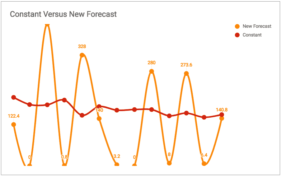
Forecasting lumpy demand brings up an issue in that it improves forecast accuracy. It means creating a highly variable forecast, as the following example from an actual client demonstrates.

Notice how a more accurate forecast (in Orange) produces enormous variability than a 12-month moving average. While the Orange line fits the demand history, it normally won’t be a desirable forecast as it will lead to a wide variance in the stock position.
Uneven Demand
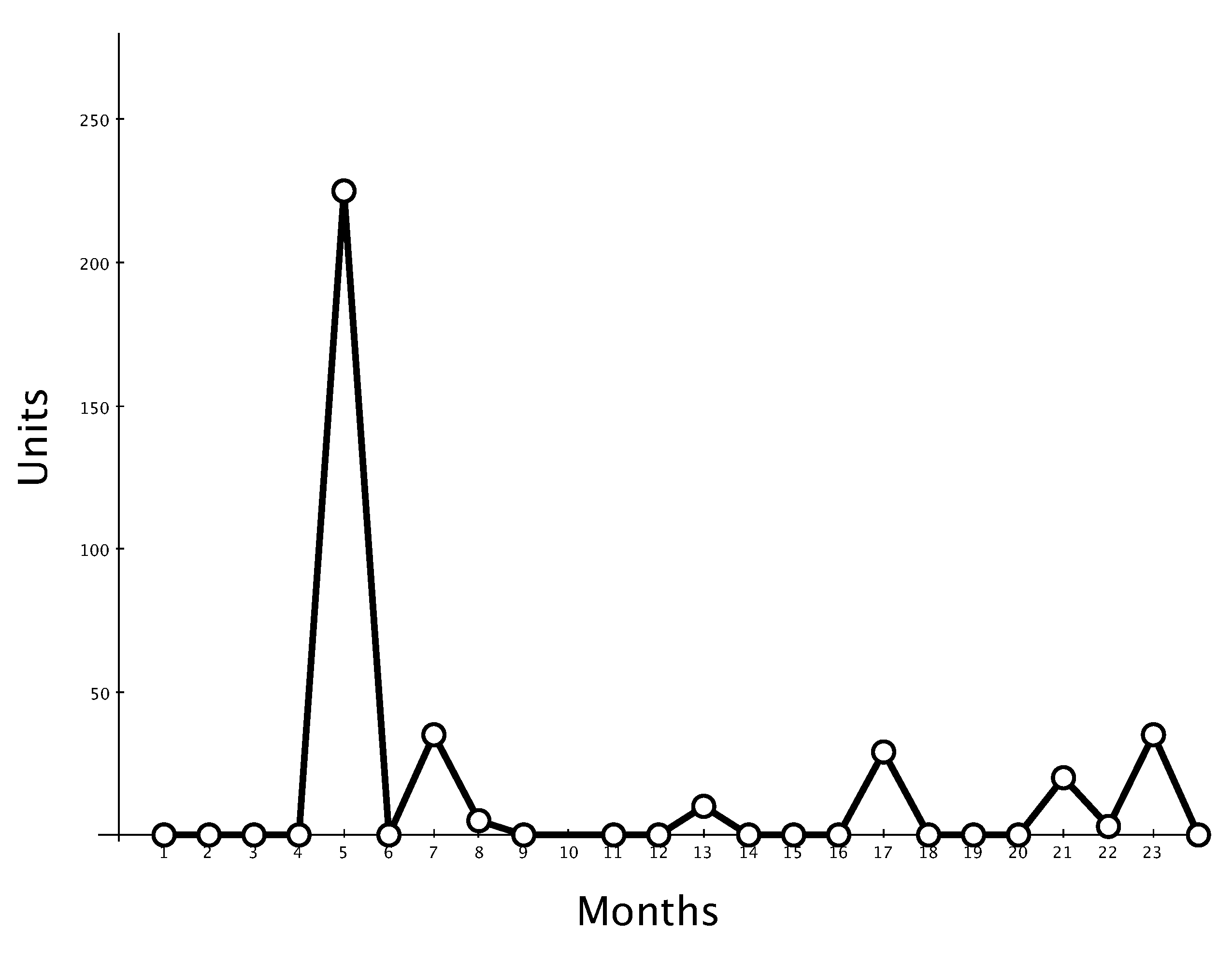
Uneven demand tends to have periods of very low or zero demand and then spikes of demand.
- There can be many reasons for uneven demand patterns. Services are part of the best-known example of lumpy demand, yet this is inherent demand.
- Service parts tend to have lumpy demand as they are based upon breakage.
- They are quite a few stocked items that have lumpy demand.
The Problem of Zero Demand History Values for Mean Absolute Percentage Error
MAPE runs into the following issues regarding calculation with zero values in-demand periods.
- The process issues around measuring forecasts are what to do when the demand or the sales history has a zero value. No forecast error can be calculated on a zero value, so the question is whether to exclude or include these data points.
- There is no forecast error when the sales period is zero, so the question is whether to exclude or include these data points.
- Research tends to be motivated to perform an inquiry for which there are easily bounded answers. This applies to the sciences as of something like forecasting.
- Papers tend to be published for those areas where there are known answers. Thus, there are many articles and writings on different prediction algorithms. However, there is little discussion on data integrity and what to do with months where demand is zero and the forecast is not zero.
What To Do with the Zero Values for MAPE Calculation
It is tough to say there is one correct answer on this topic. However, there are several alternatives.
- Ignore any items with a zero value for the MAPE
- Superimpose a forecast error over the error—for instance, 100% or 200% error for the MAPE.
- Use something called symmetrical MAPE or sMAPE.
- Eliminate the zeros by only calculating and superimposing the average sales into the periods for no demand.
- Do not divide the forecast by the actual demand. Instead, subtract them and square the result (actually removing the negatives)
The Outcomes of Each Adjustment Method
Each has different trade-offs.
- Ignoring the items with a zero value is not a valid approach for the first method as it underestimates the MAPE.
- On the second approach, if an arbitrary forecast error is superimposed upon zero demand periods, which is to say, precisely what should it be? Should it be 50%, 100%, 500%?
- As for the third method, sMAPE adjusts for zeros but then produces a value that may be useful as a relative MAPE measure but can’t be communicated well outside of the group performing the forecast error calculation. (secondly, few forecasting applications support sMAPE)
- The fourth method is eliminating zeros by superimposing the average history in months with zero demand. What this does is provide some concept of proportionality to the errors.
- The fifth method removes DIV/O error by subtracting the forecast from the demand and squaring the result to remove the negative values or simply taking the subtracted amount’s absolute value.
The sheet below shows the differences in the error calculation of the three approaches.
Forecast Error Calculation
| Row | January | February | March | April | Average |
|---|---|---|---|---|---|
| Example #1 | |||||
| Forecast | 20 | 20 | 30 | 40 | |
| Actual Demand | 50 | 0 | 50 | 0 | |
| Forecast Error (100% Error at Zero Demand) | .6 | 1 | .4 | 1 | .75 |
| Mean Demand | 25 | 25 | 25 | 25 | |
| Forecast Error (Average Demand for Periods with Zero) | .2 | .2 | .2 | .6 | .3 |
| Forecast Error by Subtraction | .3 | .2 | .2 | .4 | 110 |
| Example #2 | |||||
| Forecast | 150 | 100 | 120 | 40 | |
| Actual Demand | 300 | 0 | 50 | 0 | |
| Forecast Error (100% Error at Zero Demand) | .5 | 1 | 1.4 | 1 | .975 |
| Mean Demand | 87.50 | 87.50 | 87.50 | 87.50 | |
| Forecast Error (Average Demand for Periods with Zero) | .71 | .14 | .37 | .54 | .44 |
| Forecast Error by Subtraction | 1.5 | 1 | .7 | .4 | 360 |
*See the second example of forecast error calculation by choosing the 2nd button.
How Trader Joe’s Reduces Lumpy Demand
One company that minimizes lumpy demand on its operations is Trader Joe’s, and Why and How is a fascinating story about how active strategic decisions can improve forecastability.
They are discussed in the article How Trader Joe’s Reduces Lumpy Demand.
Where is Lumpiness in Demand History Increasing?
Many products that one would not think would be lumpy are made uneven by the company’s direct actions that they refuse to stop doing. This “unnecessary lumpiness” is primarily caused by the following:
- Sales and marketing that offer promotions
- Sales and marketing are introducing new products without culling the database for products with insufficient demand.
The general view of sales and marketing that has been communicated to me through many projects is that they should be allowed to do whatever they want as they are “helping the business.” Operations should manage around whatever sales and marketing do.
Why is Lumpiness in Demand History Increasing?
ToolsGroup, (a best-of-breed software vendor in demand and supply planning), in their white paper “Mastering Lumpy Demand,” points out that lumpiness is in general increasing. One reason for this is some products that must be planned to keep increasing. There are several grounds for this.
- A general trend in marketing is to offer more variations.
- Online retailers like Amazon.com, Netflix, and eBay are leveraging online storefronts and national distribution networks to make more selections than ever before. All one has to do to immediately grasp this is consider the demand history of a Blockbuster Video vs. a Netflix. Clearly, with so many titles, Netflix happens to have a more lumpy demand for their less popular items. I cover this in detail in my book “Supply Chain Forecasting Software.”
It increasingly appears that the more variety offered, the more variety customers demand.
As pointed out by ToolsGroup, SKUs are increasing in number faster than sales, and it’s not just in one industry. ToolsGroup attributes to more frequent replenishment more granular forecasting, and more collaboration along the supply chain. I find these second reasons less compelling than the long tail argument I will focus on in this article.
ToolsGroup’s White Paper Observations
The article also points out that even in consumer packaged goods, the long tail consumes 86% of the SKUs and nearly half the 46% of the revenue. And consumer packaged goods are not the only ones impacted.
In an electronics company that ToolsGroup worked with, 44% of the revenue was in the long tail. ToolsGroup observes that with lumpy demand, a necessary implication is the many zero-demand periods. Any attempt to improve forecast accuracy will likely be costly and useless, as it will not lead to any relevant reduction in demand variability. Instead, ToolsGroup recommends analyzing the complete probability distribution and creating a reliable statistical description of demand behavior.
*This is not an endorsement of ToolsGroup. BR&A has no relationships with any vendor.

Is Extra Complexity Managed with Systems?
Most sales and marketing types and many strategy consultants (none of whom are supply chain experts) propose that this should be no problem. The supply chain should adapt to more product proliferation and all other complexities introduced by sales and marketing. Advanced planning software, and optimizers, advanced forecasting algorithms can manage these issues. (Either that or they propose “Lean” can do it; whatever the complexity, there is, according to them, always a special band-aid that can make an inefficient business model design all better.)
The costs of all of this complexity are never calculated. As is pointed out by The Pricing Journal blog…
While many stores try to be everything to everyone, they do not realize the additional costs incurred by carrying low volume (and often negative margin) products.
The Problem With Try to Accommodate Lumpy Demand While Retaining Efficiency
Completely unknown to most strategy consultants, the less forecastable a product, the less (not more) practical advanced methods become.
Extremely lumpy products may be placed on reorder point planning, which is how planning was performed before MRP was introduced. The less forecastable items become, the less a forecast-based planning system can effectively plan them, and the more consumption-based planning without forecasting becomes a natural way to plan. Unfortunately, this is not currently happening when lumpy demand predominates for a sizable portion of the product location combinations. Instead, companies are buying into the promise of AI/ML to overcome bad SKU management practices.
Companies are essentially putting themselves in a position of having poorly performing and high-cost supply chains with large amounts of inventory and inventory obsolescence. (reorder point planning is discussed in the article How to Understand Reorder Point Planning.
Proliferation Par Excellence
There may be no better example of an industry that has gone to the extreme with unnecessary product proliferation than the grocery industry. One grocery chain takes a different path, which is a significant reason it performs so much better than the industry average.
Trader Joe’s has put itself in a better position. Fewer SKUs and fewer lower turning SKUs as a percentage of the database means that Trader Joe’s will be in a better position to have a lower forecast error, and therefore a more efficient management of their inventory than would a typical supermarket. – Supply Chain Forecasting Software
Going Against the Grain in Reducing Lumpy Demand
Trader Joe’s does something unusual in this day and age. They have operations with a place at the table, co-developing the strategy and policies with sales and marketing.
How is this possible?
Sales and marketing (primarily at the food companies, which control supermarkets’ theme and orientation) have turned most supermarkets into packed to-the-gills, plastic environments with massive product proliferation. They are quite unappealing places in which they shop, and they also have high forecasting and supply chain costs. Sales and marketing drove these decisions, with the idea that the more items were offered, the higher the sales.

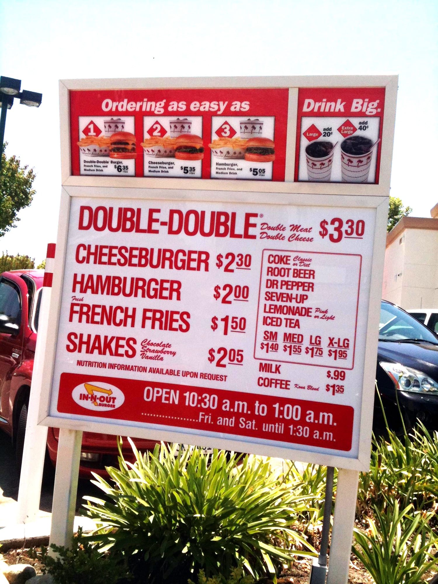
The restaurant with the most extended lines in the US also happens to be the one with the most limited menu.
This video shows what a “terrible” company In n Out Burger is. N Out Burger is saddled with overcrowded locations, cities that call up In-n-Out Burger and ask them to open a store in their area, the highest employee satisfaction in fast food, and one of the highest loyalty followings of any fast-food franchises.
Is it Time for In n Out Burger to Listen to Marketing?
These burdens could all be reversed if only In n Out Burger would listen to marketing experts to proliferate their menu and massively decrease their operation efficiency.

Once again, marketing can’t seem to find the existence of any of these successful companies.
Marketing Illustrates How to Ignore the Data Points of Successful Low SKU Environments
Whenever a company successfully contradicts the official storyline of sales and marketing, sales and marketing confidently ignore the example.

Trader Joe’s has had great success with a smaller number of higher-turning SKUs in their stores. However, according to sales and marketing, this is not possible, and therefore, they ignore Trader Joe’s. Trader Joe’s also does very little marketing, and its popularity is more based upon in-store experience. It offers a better in-store experience by paying the people who work in the store more than large grocery chains and having fewer people in marketing. Trader Joe’s employees often look happy to be working there, unlike many employees of large chain stores who can sometimes appear to be on suicide watch.
Because this is offensive to marketing, they won’t talk about Trader Joe’s. If stores were managed more like Trader Joe’s, there would be many unemployed marketing people. Some of them may have to switch careers and get a real job doing real work — for instance, working in Trader Joe’s. Never repeat this to a person in marketing, as you might get punched.
Maximizing SKUs and Minimizing Freshness
Recovering these costs means offering more varieties of processed foods, which have higher margins and can sit longer due to their elevated preservative levels. If your inventory turns are slow because you have proliferated your product database, you cannot afford to keep a significant percentage of fresher food.
On the other hand, by designing a simpler model, Trader Joe’s finds itself in a positive feedback loop. It can keep its prices low (for a better product even) because its supply chain efficiency is higher than the industry average.
Trader Joe’s can offer a freshness level in its food that the significant supermarkets simply can’t.
Comparing Different Methods
A study by the Decision Sciences Institute examined the following standard lumpy demand forecasting methods.
Simple Moving Average
Single Exponential Smoothing
Croston’s Method
SBA (Syntetos and Boylan) Method
This research found the SBA method to be superior to the other three methods. The book Complex System Maintenance by Murthy and Kobbacy also found that the SBA method was superior to the SMA, SES, Croston’s method. The SBA is a bias-corrected adaptation of Croston’s estimator. These were used to predict 3000 service parts from the automotive industry. Other publications question whether SBA is all that superior to Croston’s. One such article is “On the Bias of Croston’s Forecasting Method” by Ruud Teunter and Babangida Sani. They propose that the negative bias of SBA is greater than the positive bias of Croston’s.
In our analysis, these methods tend to provide a mask for the problem. The problem is that the demand is difficult to forecast, and the error will be high no matter what forecasting method is used. Simple, intermittent demand does not have a good pattern, and statistical methods are based upon pattern recognition.
Bucketing Products
One of the most important steps in dealing with lumpy demand is segmenting the products into lumpy buckets and those that are more stable and consistent. This is because a forecasting algorithm that works very well for lumpy demand will seldom work well for steady demand, and while much of the product database may be lumpy, most likely not all of it is. Another issue is the low-demand items. Lumpy low-demand items should go out on the service parts forecasting algorithm.
Forecastability
Many products are not forecastable. That is, no statistical forecasting procedure can defeat a naive forecast. I have developed a formula (with a previous client) that can be applied to a product database to determine which products or product location combinations are forecastable.
Reviewing Intermittent/ Service Parts Error Measurements and Safety Stock Literature
We specifically searched for dynamic safety stock with error measurements that work with forecast errors that can handle zeros in the demand history like MASE & MAAPE, which we use in the Brightwork Forecast Explorer Error Calculator. We used an academic search engine that reliably finds such articles. We found little there. Quite the opposite, the items assume that the error measurement like MAPE that cannot be used with lots of zeros is applicable for most companies.
Now, there are methods published for calculating safety stock dynamically in a service parts environment, but they are complicated. In reviewing them, we don’t think they would migrate well to a real environment. They are more academic curiosities, primarily used to show off math talent by the academic authors rather than create a usable method for the industry.
Conclusion
There is weak evidence that more sophisticated methods beat simple methods at forecasting for products with lumpy demand. Secondly, more advanced methods consume much more time and effort from the company, so while the results do not improve with complex methods, the maintenance effort always increases. As a practical matter, it is hard for me to see why so much effort has been spent in the forecasting literature attempting to forecast products with such erratic histories.
The central concept to statistical forecasting (as opposed to consensus prediction, which is based on judgment and domain expertise) is that there is a pattern that can be used by the forecast algorithm that is selected. If a demand history does not have this, it makes little sense to apply more sophisticated methods. This is a critical point in determining how to deploy forecasting resources.
Trader Joe’s follows a grand strategy; while it is infinitely logical, it is a strategy that few companies inside or outside the grocery industry can copy. One primary reason is that sales and marketing are too robust at most companies to allow rational decisions from a supply chain perspective to be rolled out.
Like Southwest Airlines (another company with sky-high customer satisfaction), robust sales and marketing departments in competing airlines cannot allow their airline to copy a successful approach. It would reduce their control over their company’s policy.
In the aviation and grocery industries, operations must be kept in their place, and sales and marketing must be allowed to have their way in all decisions. In most companies, supply chain management is now merely an order taker for sales, marketing, and finance.
- Lumpy demand is a function of stocking decisions primarily controlled by the sales strategy.
- Lumpy demand is the most difficult to forecast, translating into a high stock level per the mean demand.